- INTRODUCTION
Grape is sub- tropical crop in India which belongs to Vitaceae family(National Horticulture Board, n.d.). In India total production of Grapes is 1,234.9 thousand tons in an area of 111.4 thousand ha which occupies around 2% of world’s production with a productivity of 11.1 tons/ha. Total export of grapes from India is 108.58 thousand tons during 2011-12 (AgriXchange). 17-20% of grape production is used for drying, 0.5% is used for wine production, 1.5% is for juices and rest is used for table purposes whereas USA and Turkey together contributes 80% raisins production in World (P.G. Adsule, 2007).Fresh grapes from India is exported to 30 countries.
Problem Definition
Due to low shelf life of grapes, the removal of moisture from grapes is needed to a certain level for the preservation of raisins over an extended period of time. Using traditional methods, time period for drying is long and the quality of raisins produced in India is not marketable and non-exportable. Efforts are needed to improve the quality of raisins, lower the costs of drying and reduce the period of drying. Computational fluid dynamics is required for the designing of cabinet in drying setup to predict the uniform flow of air and velocity .
Literature Survey
An experimental setup is designed for the study of convective drying to achieve a maximum velocity of 8m/s and temperature of 70°C and experimentations are performed(Mohan & Talukdar, 2013).Design and construction of various types of solar dryers is reviewed by (Ekechukwu & Norton, 1999). (Augustus Leon, Kumar, & Bhattacharya, 2002) reviewed the methods used for evaluation of solar dryer and compared the results obtained using different methods based on the results they proposed the comprehensive procedure for evaluation of dryer.
Experimentation of drying involves three processes pre-processing, drying and post-processing (Esmaiili, Sotudeh-Gharebagh, Cronin, Mousavi, & Rezazadeh, 2007).Thompson Seedless grapes are used for drying which is brought from Sahyadri Farms, Nashik. Pre-treatment of grapes is done using Ethyl Oleate solution containing 25% of K2SO4. Using the different models and drying kinetics the effects of pre-processing and post processing is reviewed by (Esmaiili et al., 2007)
Different types of models proposed for drying kinetics are reviewed by(Doymaz, 2012) and the results obtained are compared.
- THEORY
- Drying Theory
Removal of moisture from a substance due to simultaneous heat and mass transfer known as Drying. When the continuous air is supplied to the solid, the point where vapour pressure of the moisture of solid become equal to partial pressure of the vapour i. e. solid and gas are said to be in equilibrium with each other and the moisture content of solid is known as the equilibrium moisture content which depends upon particle size and specific surface. Equilibrium is generally achieved due to adsorption (evaporation) or desorption (condensation).
Types of Moisture :
- Bound Moisture : The equilibrium vapour pressure of the moisture contained by solid becomes less than that of pure liquid at the isothermal conditions is termed as bound moisture.
- Unbound Moisture : When the solid moisture exerts an equilibrium pressure equal to that of pure liquid at isothermal conditions is known as Unbound moisture.
- Equillibrium Moisture : The moisture content of substance becomes in equilibrium with a given partial pressure of vapour is known as equilibrium moisture.
- Free Moisture : The moisture contained by the substance in excess of the equilibrium moisture is known as free moisture.
Figure 1 : Moisture content versus Relative humidity curve for different types of moisture
Type of dryer use is generally depends on :
- Method of operation : Batch or continuous
- Method of supplying heat : direct contact or indirect contact
- Nature of substance : rigid or flexible
Parameters which are generally considered for a dryer are :
- Physical Properties of dryer
- Size, shape and type of dryer
- Loading density and the ease in loading/unloading
- Number of trays and its area
- Thermal performance
- Drying Rate
- Airflow rate, Temperature and Relative humidity
- Dryer efficiency
- Quality of dried product
- Colour , flavour and texture
- Nutritional attributes
- Economical evaluation (cost and payback period)
Rate of Drying Curve :
Figure 2 : Rate of Drying curve for constant drying conditions
In figure 2, region A-B represents the rise in surface temperature to ultimate value to attain equilibrium if surface is colder and if the surface is hotter than it is vice versa. B-C represents removal of unbound moisture from substance and is known as constant drying period. Constant rate period continues till the water present on the surface of the substance gets evaporated i.e. water evaporates becomes equal to the amount of water supplied. Then the falling rate period starts i.e. drying rate starts falling down. First falling rate period is known as the Unsaturated surface drying, it occurs when wetted solid spots continuously start decreasing till its dried i. e. it arrives at point D. Second Falling rate period is from D to E which is internal movement of moisture controls. Heat required for moisture removal is transferred through the solid to the vaporization of water in the solid and the vapor moves from solid to the air stream.
- CFD TheoryReynolds Transport Theorem
The relation between system equation and control volume is given by Reynolds Transport Theorem. It is easier to work with Control Volumes instead of identifying and following a system of fluid particles. Reynolds Transport equation is as follows:
Term 1 : Rate of change of Extensive Property
Term 2: Rate of change of the amount of property N in Control Volume
Term 3: Net flux of N through the Control Surface
- Navier Stokes Equation
Navier stokes equation describes the relation between velocity, temperature, pressure and density of a moving fluid. The effects of viscosity are also included. These are called coupled system of equations. Navier Stokes Equations are valid as long as representative physical length of a system is much larger then the mean free path of molecules(n.d.).
Mass Balance or Continuity Equation
Equation of Mass balance in any element of fluid is:
Term 1 : Rate of change of density
Term 2 : Divergence of the mass velocity vector
Continuity equation for incompressible fluids :
Momentum Balance or Equation Of Motion
The Momentum balance equation is as follows:
Energy Balance Equation
Basic concept of energy balance equation is as follows:
Where,
- Schemes and Discretization
Properties of discretization includes:
- Conservativeness : A set of discretised equation is solved for the conservation of transport property, F. The flux of F leaving the control volume of a certain face must be equal to the flux of F entering the adjacent control volume through the same face.
- Boundedness : Scarborough criteria i. e. for convergent iterative methods a certain conditions are provided in the form of equation:
Other essential condition for boundedness is all coefficients which are involved in the equation should have the same sign (generally positive).
- Transportiveness : It determines the direction of flow or the strength of convection relative to the diffusion.
The general form of discretised equation for 1-D, 2-D and 3-D diffusion problems is:
The following schemes can be applied to solve CFD problems(an-introduction-to-computational-fluid-dynamics-versteeg.pdf, n.d.):
| Schemes | Properties | Drawback |
| Central Differencing Scheme | – Diffusion dominant – Average of neighbouring nodes is considered in equation i. e. Fe = (FP+FE)/2 and Fw = (FW+FP)/2 -second order accurate | – combined effect of convection and diffusion cannot be considered in depth – not able to identify flow direction -unstable |
| Upwind Differencing (Donor cell) Scheme | -Convection dominant -Accounts the flow direction – Convected value of F is taken to be equal at the upstream node i. e. for positive direction Fw=FW and Fe=FP For negative direction: Fw = FP and Fe=FE | -accuracy is only first order due to backward differencing formula -Exact solutions cannot be obtained due to False diffusion |
| Hybrid Differencing Scheme | -Combination of central differencing scheme(Pe < 2) and upwind differencing scheme(Pe ³2) -highly stable compared to higher order schemes | -Exploits the favourable properties of the upwind and central differencing scheme |
| Power law Scheme | -Similar to hybrid differencing scheme -Diffusion is negligible when Pe exceeds 10 – when 0 < Pe < 10 polynomial expression is used to evaluate flux | – For 1-D it gives more accurate exact solution compared to 2-D and 3-D. |
| QUICK (Quadratic upstream interpolation for convective kinetics) Scheme | -Uses a three-point upstream weighted quadratic interpolation – for calculating flux 2 downstream and 1 upstream node is included | – can be unstable due to negative coefficients |
The examples given in (an-introduction-to-computational-fluid-dynamics-versteeg.pdf, n.d.) is solved using MATLAB.
- Turbulence Modelling
Turbulence possess unsteady and chaotic features in 3-D with strong diffusivity having a wide range of eddy sizes due to which energy cascading occurs (vortex stretching process) which is strongly non- linear, non-integrable and non-Gaussian.
The flow through close conduits and jets give arise to two classes of flow which are called as wall turbulence and free turbulence.
Physics of turbulence includes:
- Eddies
- Fluctuations
To get the accurate results an extremely fine mesh size is required with very small size time step which is impossible in realistic engineering problems . To overcome this issue, concept of time averaging in Reynolds Averaged Navier Stokes(RANS) Equation is introduced. RANS equations can be derived from the equations of Mass, Momentum and energy equations by substituting Reynold’s Decomposition Equation i. e. , , and
Mathematical models are developed to predict the effects of turbulence. Following are the commonly used models
- Standard k-ε model
The Equations of k-ε model are derived using momentum fluctuation equation are as follows:
Exact k equation:
Modeled k equation (Using Assumptions) :
In exact k equation Term I represents rate of change of k, Term II represents convective transport of k by the mean velocity field, Term III represents turbulence production due to interaction of Reynold’s stresses with mean velocity gradients, Term IV represents transport of k due to interaction of fluctuating velocity and fluctuating pressure, Term V represents transport of k by fluctuating velocity, Term VI represents transport of k by molecular viscosity, Term VII indicates destruction of k by action of molecular friction.
Exact ε equation :
Modeled ε equation(Using Assumptions):
In exact Equation, Term I represents the time rate of change of ε, Term II indicates convection of ε by mean flow velocity field, Term III and IV is the production of ε by the deformation of mean flow field, Term V denotes the production of ε by the gradient of mean vorticity, Term VI represents the production of ε by the gradients of fluctuating velocity or vortex stretching, Term VII indicates turbulent diffusion of ε by the fluctuating velocity field, Term VIII denotes diffusion of ε by interaction between gradients of fluctuating velocity and fluctuating pressure, Term IX represents the diffusion of ε by molecular viscosity and Term X is the destruction of ε by the action of molecular viscosity.
- Hands on Tutorials And SimulationsTutorialsCavity(OpenFOAMUserGuide-A4.pdf, n.d.)
Figure 3 : Geometry of the lid-Driven cavity
The geometry is shown in figure 1 (2-D) the upper wall is moving at the velocity of 1m/s and rest all the walls are stationary. Icofoam solver is used for laminar, incompressible and isothermal conditions whereas pisofoam is used for turbulent, isothermal and incompressible flow. The effect of mesh resolution and mesh grading is investigated.
Increase in grid size gives the better visualization of flow inside the cavity. 80X80 grid gives the bogus result due to the increase in grid size more than it can handle. Similarly results are compared for decreasing kinematic viscosity for 20X20 grid and it is observed that as it decreases the turbulence increases due to increase in Reynolds number and the visualisation of flow inside cavity decreases.
- Duct (“Mark Kimber – YouTube”)
Figure 4 : Geometry of duct
The geometry shown in figure 3 (3-D) having dimensions as 0.2m x 0.5m x 0.5m is simulated using the simplefoam solver for incompressible flow of fluids.
The simulations on duct is performed for different mesh resolution and the data obtained is post- processed to find the Fanning friction factor and Moody friction factor. The values of fanning friction factor and Moody fraction is compared with expected value and error is determined.
- Simulations of Dryer DomainGeometry of Dimensions and scale
Drying of grapes in large scale which is generally done by farmers using air draft method. Shed is provided above the dryer. Dimensions of dryer are 100ft x 5ft x 12ft for loading 3.6 tonnes of grapes per batch. The racks which are placed inside the dryer have dimensions as 100ft x 5ft x 1ft (in z-x-y direction)with distance between each rack as 1ft. 5 inlets are provided of dimensions 5cm x 5cm at equal distances on the face having dimensions as 5ft x 1ft (x-y direction). Similarly, at 100ft in z direction on the face of 5ft x 1ft, 5 outlets are provided having dimensions as 5cm x 5cm because the lowest area of fan available is 45 x 72 mm2 which gives the side of around 50mm.
Figure 5: Geometry of Rack Single Tray
- Pre-processing /Meshing
9 different grids sizes are created using GAMBIT among them 5 geometries are of different types:
Type 1 : 5ft x 1ft (in x-y direction) inside which 5 more faces are created (inlets) and an edge along y direction is created. All the faces and an edge are meshed and extended to the volume with mesh.
This type of geometry is used for four different grid sizes : 1,60,000 ; 3,50,000 ; 6,05,000 ; 8,50,000
Type 2 : This geometry is similar to type 1 meshing pattern is changed. In this boundary layer type mesh is created on boundaries if the front and back faces and for rest of the geometry hex mesh is created.
This type of geometry is used for grid size of 1,25,000.
Type 3 : : 5ft x 1ft (in x-y direction) inside which 5 more faces are created (inlets), at the distance of 30mm in z direction face of 5ft x 1ft created and corresponding edges and faces created, all these combined to create 1 volume. At a distance of 29,940mm mirror image of volume 1 is created and at the middle part corresponding edges and faces are created. For volume1 and mirror image of it is meshed with hex/tri whereas middle part is meshed with hex.
This type of geometry is used for grid size of 2,72,387.
Type 4 : This is similar to geometry 1 meshing is changed. On face with 5 inlets hex/tri mesh is created whereas for entire volume hex mesh is used.
This type of geometry is used for two different grid sizes :
Type 5: This geometry is similar to geometry 3 meshing is done in different way. All faces are meshed with hex whereas volumes are hex/tri(here front face is and back faces not taken in volume).
This type of geometry is used for grid size of 2,72,387.
Type 1 Type 2
Type 3 Type 4
Type 5
Figure 6: x-y face meshes for each type of geometry
- Test Cases
The grid sizes obtained are simulated for the kinematic viscosity of 1e-3, 1e-4and 1e-5 for 0.3m/s of velocity, then velocity is changed to 0.6m/s, 1m/s, 3m/s and 9m/s. Geometry is visualized using ‘Para-View’ software and corresponding pressure drop and mass flow rates are obtained. Using the data obtained energy balance and mass balance is calculated.
- Post-processing
- Mass Balance vs Grid Size for different veocities
- Jet length vs Velocity for different Grid Size
- EXPERIMENTATION
- Objective
and Experimental Setups
- Traditional Methods
- Objective
and Experimental Setups
Traditional Methods of drying includes Stand Dryer which are classified on the basis of type of trays i. e. (i) Net Tray Stand Dryer
(ii) Mesh Tray Stand Dryer
(iii) Solid Tray Stand Dryer
Objective : To confirm drying time and replication of traditional methods using Net Tray, Mesh Tray and Solid tray.
Experimental Setup
The experimental setup contains three rectangular trays parallel to each other having dimensions as 50cm*50cm. The distance between each tray is 1 foot. The distance after last tray is 1 foot and before 1st tray is 1 foot i.e. total height of the setup is 5 foot. At the top of the setup shed is provided. From sides the setup is covered with net to allow the air flow .
Net trays are made up of Nylon anti-bird protection net. Mesh trays are made up of iron with thickness of 0.8 mm punched Mesh whereas Solid trays are made up of Mild Steel with thickness 0.8mm.
Mild Steel 0.8mm Punched Mesh 0.8mm Nylon Anti-Bird Net
Figure 7 : Experimental Setup for traditional Drying
3.1.2 Solar Dryer
Objective : To develop a low cost drying
Experimental Setup : There is semi spherical dome structure built by research fellows in Vigyan Ashram, Pabal. They claimed that “ Semi spherical shape is better for drying efficiency” (No quantitative data as an evidence is available from their side). Details of structure are as follows:
| Trays | Area | Proportion |
| 1 | 1.99E+5 | 1 |
| 2 | 4.68E+5 | 2.35 |
| 3 | 6.77E+5 | 3.40 |
| 8.26E+5 | 4.14 | |
| 5 | 9.46E+5 | 4.74 |
Figure 8 : Experimental Setup of Dome Dryer
3.1.3 Lab-scale Electrical Dryer
Objective : To determine the optimum flow rate and temperature for drying using air draft method and to check non-uniformity.
Experimental Setup : An FRP box of 50cm by 50 cm by 35cm was fabricated with 40 staggered inlets per tray were made of 5 mm size so as to get a uniform flow. A 250 watt centrifugal blower was installed, with conical inlet and outlet at either ends of the dryer so as to facilitate unconstrained movement of air. A 5 kW heater was installed considering a maximum temperature of 85oC and maximum flow rate of 500 m3/hr. The 0.5 mm mild steel conical inlet and outlet ducts were insulated with FRP. A K-type thermocouple was installed for a PID controller to maintain its temperature.
Net trays were also used for experimentation. Tray were made using, a 6 mm MS bar bent into a square shape and welded at the open corner. Nylon anti bird net was fastened to all sides, and bunches were kept on the net.
Figure 9 : Experimental setup of pilot dryer
3.2 Design of Experiments
Grapes are pre-processed at 40°C, they are kept in ethyl oleate solution having 25% K2SO4 in it (1.8 litre in 100 litres of water) for 3 minutes to remove the waxy layer present on grapes. In case of traditional methods of drying and lab scale electrical dryer 3kg, 6kg and 9kg of grapes batches we have kept for experiment, equal amount of grapes are placed in each tray. In case of dome dryer 15 kg of grapes are arranged according to the proportion given in table shown with diagram.
- Sampling Techniques
Ambient RH and Temperature is measured. In case of solar dryer and lab scale electrical dryer the RH and temperature of exhaust is also measured. Samples are taken from the bottom tray everyday at the interval of 12 hours. In case of Dome Dryer weight of 1 tray from each rack is also measured to determine the weight of water lost from every rack. Sample is weighed and kept in electric oven till it becomes moisture free. The dried sample in oven weighed and loss on drying is determined.
- Data Analysis
Traditional Methods
Net Tray vs Punched Mesh Tray vs Tassgaon Net
Figure 10 : Graph of Tassgaon pattern using different trays
It is observed that mild steel solid trays loaded with berries provide better drying as compared to loading of bunches on nets. It can also be observed that with a flow rate corresponding to 3m/s i.e. 38m3/hr drying time can be reduced to almost half.
Pilot Dryer
- Drying Time vs Velocity(3,6,9 m/s)
For 3 kg of batch, the resulting time for the velocities 3m/s, 6m/s and 9m/s are respectively 190, 125 and 95 hours.
Figure 11 : Graph of Pilot Dryer for velocity Comparison
It can be concluded that with increase in velocity, drying time can be reduced. However, an optimum flow rate needs to pin pointed, where the drying time as well as the flow rate in lowest so as to saving cost of pumping power.
- Drying Time vs Temperature(40°C , 55°C)[For Net Trays]
40oC was selected as a minimum temperature as the ambient temperature was around 39oC to 43oC during afternoon. Maximum temperature selected as 55oC to avoid browning of grapes, with a constant velocity of 3m/s (38m3/hr flowrate).
Figure 12 : Graph of pilot dryer for temperature comparison
It can be seen very clearly that increase in temperature results in faster drying rate. Drying time required to get to approximately 10% moisture content is reduced from 160 hours for 55oC to 100 hours for 40oC. However, more temperatures in the range of 40oC to 55oC need to be experimented to ascertain the nature of this trend.
- Drying Kinetics
Applying Fick’s law for drying and assuming effective diffusivity and neglecting edge effect gives second order differential equation as follows:
Where, X is the moisture content, t is the time and Deff is the effective moisture diffusivity. This equation is further solved to derive the Page model equation(Margaris & Ghiaus, 2007) :
Where, X -average moisture content, Xe is equilibrium moisture content, Xi is initial moisture content, K and N are product constants which are evaluated for Thompson Seedless grapes in (Azzouz, Guizani, Jomaa, & Belghith, 2002) gives :
As calculated in (Azzouz et al., 2002); , ,
, ,
Substituting these Values K and N are obtained as 4.05e-4 and 0.9326.
Experimental and Page model graphs have been compared for 3m/s at 40°C:
It can be clearly seen from the equation of graphs that there is large difference in the coefficients obtained from equation of experimental and page model and it can also be observed that page model is second order polynomial whereas results obtained experimentally gives fourth order polynomial which makes a huge difference and it can be concluded that page model does not satisfies experimental results obtained .
- CONCLUSION
Drying period of almost half the time of Tassgaon method is achieved using the air by draft i.e. lab scale electrical Dryer. Results obtained from experiments using traditional method using Solid trays, punched mesh trays and Net trays are compared. Also for solar dryer open sun drying and shed drying results are compared and for pilot dryer results are compared for different flow rates and also for temperature of 40°C and 50°C.
For Simulations graphs obtained for mass balance vs grid size for different velocities are seen. Also effects of jet length have been observed.
- FUTURE WORK
- Simulations to study non-uniformity in traditional setup
- Different kinetics models to be compared with experimental results.
- Design of a drying setup for commercial scale use.
- Economical evaluation and cost estimations for commercial scale dryer.
- Incorporation of solar energy and dehydration systems for faster drying at lower costs
- REFERENCES
an-introduction-to-computational-fluid-dynamics-versteeg.pdf. (n.d.). Retrieved from https://ekaoktariyantonugroho.files.wordpress.com/2008/04/an-introduction-to-computational-fluid-dynamics-versteeg.pdf
Augustus Leon, M., Kumar, S., & Bhattacharya, S. C. (2002). A comprehensive procedure for performance evaluation of solar food dryers. Renewable and Sustainable Energy Reviews, 6(4), 367–393. https://doi.org/10.1016/S1364-0321(02)00005-9
Azzouz, S., Guizani, A., Jomaa, W., & Belghith, A. (2002). Moisture diffusivity and drying kinetic equation of convective drying of grapes. Journal of Food Engineering, 55(4), 323–330. https://doi.org/10.1016/S0260-8774(02)00109-7
Doymaz, İ. (2012). Sun drying of seedless and seeded grapes. Journal of Food Science and Technology, 49(2), 214–220. https://doi.org/10.1007/s13197-011-0272-9
Esmaiili, M., Sotudeh-Gharebagh, R., Cronin, K., Mousavi, M. A. E., & Rezazadeh, G. (2007). Grape Drying: A Review. Food Reviews International, 23(3), 257–280. https://doi.org/10.1080/87559120701418335
Margaris, D. P., & Ghiaus, A.-G. (2007). Experimental study of hot air dehydration of Sultana grapes. Journal of Food Engineering, 79(4), 1115–1121. https://doi.org/10.1016/j.jfoodeng.2006.03.024
Mark Kimber – YouTube. (n.d.). Retrieved July 5, 2019, from https://www.youtube.com/channel/UCE2C6rXiC62TICNIwHtiYoQ
Mohan, V. P. C., & Talukdar, P. (2013). Design of an experimental set up for convective drying: Experimental studies at different drying temperature. Heat and Mass Transfer, 49(1), 31–40. https://doi.org/10.1007/s00231-012-1060-4
OpenFOAMUserGuide-A4.pdf. (n.d.). Retrieved from http://foam.sourceforge.net/docs/Guides-a4/OpenFOAMUserGuide-A4.pdf
P.G. Adsule. (n.d.). (10) (PDF) Raisin Production in India. Retrieved July 6, 2019, from ResearchGate website: https://www.researchgate.net/publication/265089071_Raisin_Production_in_India
What Are the Navier-Stokes Equations? (n.d.). Retrieved June 30, 2019, from https://www.comsol.co.in/multiphysics/navier-stokes-equations